(Written by Jonathan Sheppard and Aaron Conover)
This summer, Jon Sheppard and Aaron Conover joined Merideth Frey’s physics research team through the Sarah Lawrence Summer Science Internship program. Last summer, the team focused on setting up the new TeachSpin equipment and optimizing the Halbach Mandhala design. They were successful in both endeavors. Thus, this summer, the attention has been on designing and creating a Radio Frequency transceiver and an easily manipulated gradient field (while also attempting to optimize all magnetic fields even further).
Jon took on the creation of the RF transceiver while Aaron got to work on the gradient field and its manipulation mechanism.
RF Probe
Below is a diagram of the circuit Jon used in his design. This circuit is based on the tank circuit given in the book Experimental Pulse NMR: A Nuts and Bolts Approach by Eiichi Fukushima and Stephen B. W. Roeder.
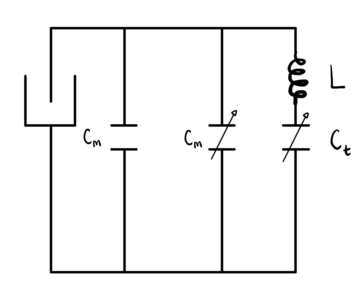
In addition to the circuit, we also had to come up with the specifications of the inductor coil itself. To this end, we coded a Python script that, when given a few baseline numbers, would calculate the rest of the necessary values.
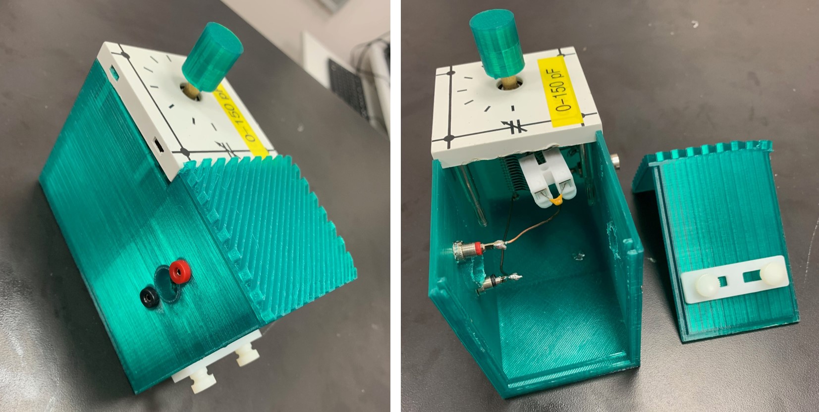
The tank circuit enclosure manifested itself in two variations. In the first attempt, we designed and used a 3-D printed enclosure. After a few drafts, we made one that we liked, and went forward with implementing the circuit within the enclosure. Pictured below is the final result.
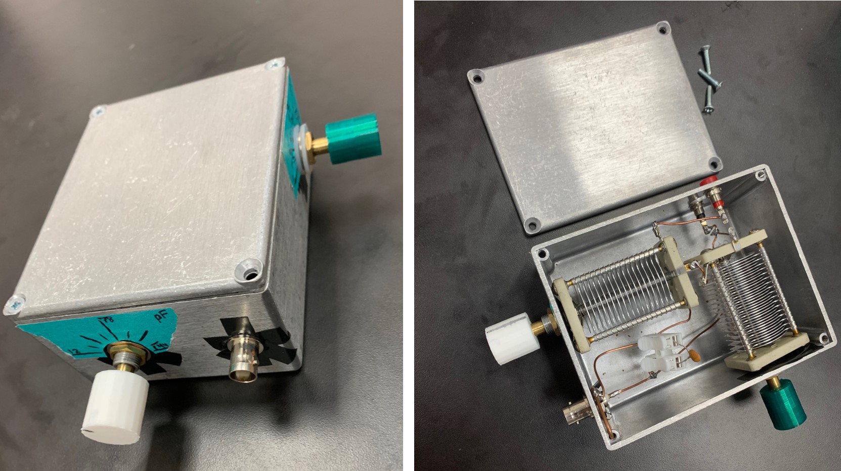
But then we noticed a lot of background noise coming from the transceiver. In an attempt to lessen this noise, we tried to recreate the circuit in an aluminum box. We bought more variable capacitors so the first transceiver could remain intact, and we created a second with the aluminum enclosure. The first version of this metal upgrade wasn’t captured in a picture before we modified it yet again. However, in the second version (picture below), the only difference is we added a variable capacitor in parallel to our static matching capacitors.
We then tested these systems extensively. As stated previously, we noticed a lot of noise coming from the 3-D printed enclosure. When testing the aluminum enclosure, we noticed a similar amount of noise. In order to reduce this, we designed and built some rudimentary shielding, which brought our noise levels equal to that of the manufactured TeachSpin system.
Magnetic Gradient Creation
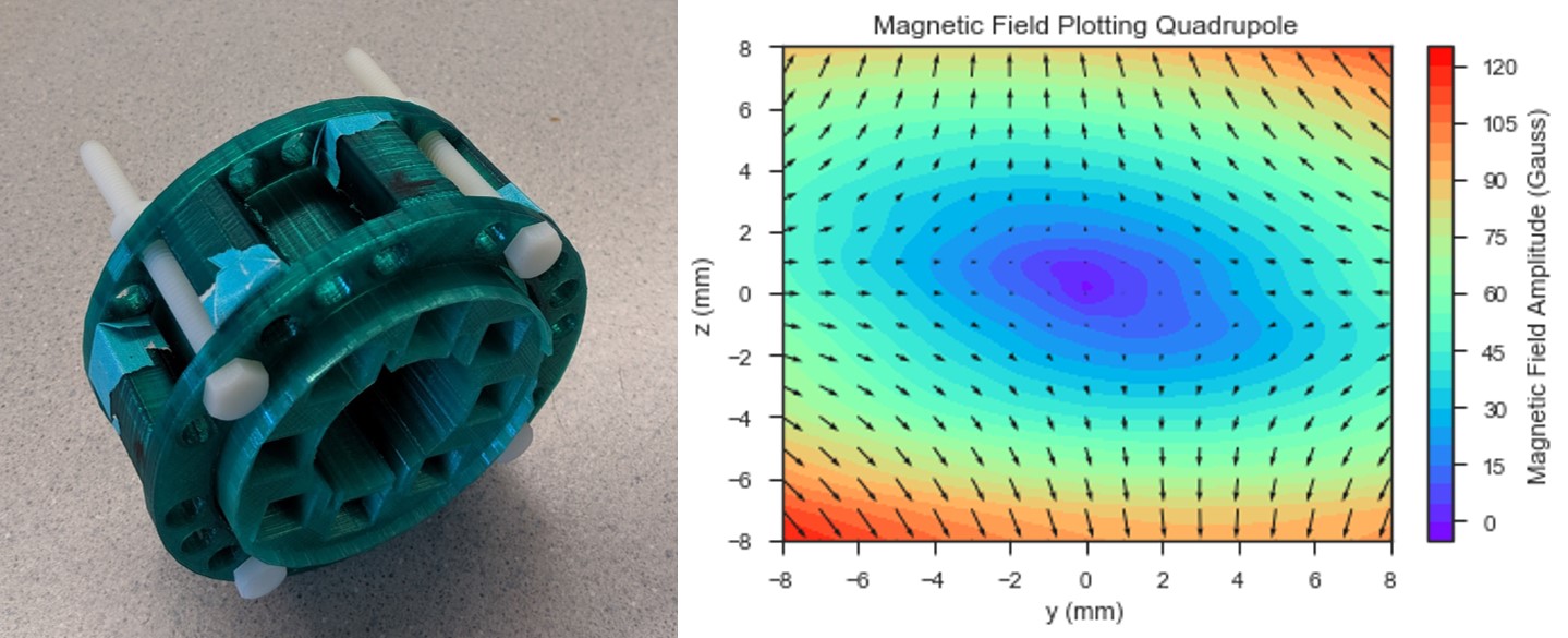
Concurrently, we were designing an improved system for manipulating our gradient. The initial plan was to rotate the gradient magnets using a servo and Arduino board, allowing us to manipulate it to the degree. However, this presented potential problems in rotating the gradient, which is on the exterior of the mandhala, while not hindering any flow tubes that would be used to keep the zebrafish inside alive. As such, we switched to using the servo to rotate the sample, by using a 3d printed drill chuck to hold the test tube. The gradient magnets are now adjusted manually using a new gradient setup that had holes along the rings every 15 degrees, excluding multiples of 90, as those are occupied by the magnet holders. This will allow us to manipulate the gradient manually which, while not as ideal as having control down to the degree of the gradients, will service us with not too much extra work when combined with rotating the sample tube. This project made extensive use of AutoCAD to create the structures used, as well as FEMM to ensure a homogeneous magnetic field.
For the final 3D print files we created, see the Thingiverse page.
After the new gradient was printed, we used a gaussmeter to collect specific values of magnetic induction across the inside of the gradient in all 3 configurations, along the 2D cross-sectional plane at the center of the magnets. This data, when processed, showed that, while not all of the configurations were ideal, the strongest central configuration conformed to our expectations of a quadrupolar magnetic field, and provides a linear gradient of ~11 Gauss/mm.
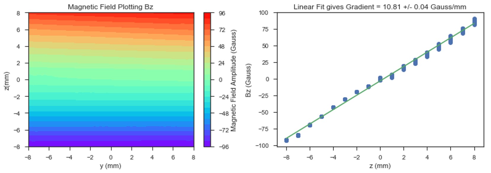
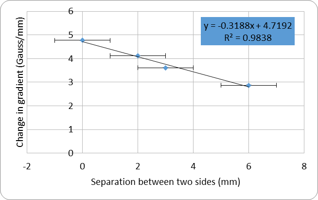
Building off of the gradients already used, the next step was to print two more gradient magnet holders to form the gradient along the cylindrical axis. Unlike the previous gradient, these holders will have magnets in the same configuration as the NMR Mandhala. Between the two gradients, one placed with its field in line with the Mandhala’s field and the other placed to oppose the Mandhala, means that we can achieve a difference in field strength of the Mandhala as you move from front to back, producing a good linear gradient that will be useful when we begin imaging. Once again, the gradient created by this apparatus was measured and graphed to show that it is a linear change across the length of the Mandhala. It provided a maximal gradient of ~5 Gauss/mm when the two holders are right next to each other, and the gradient strength goes down as they are separated (see plot below.) Even with minimal separation, the gradient had great linearity over the 20 mm in the center where the sample would be placed.
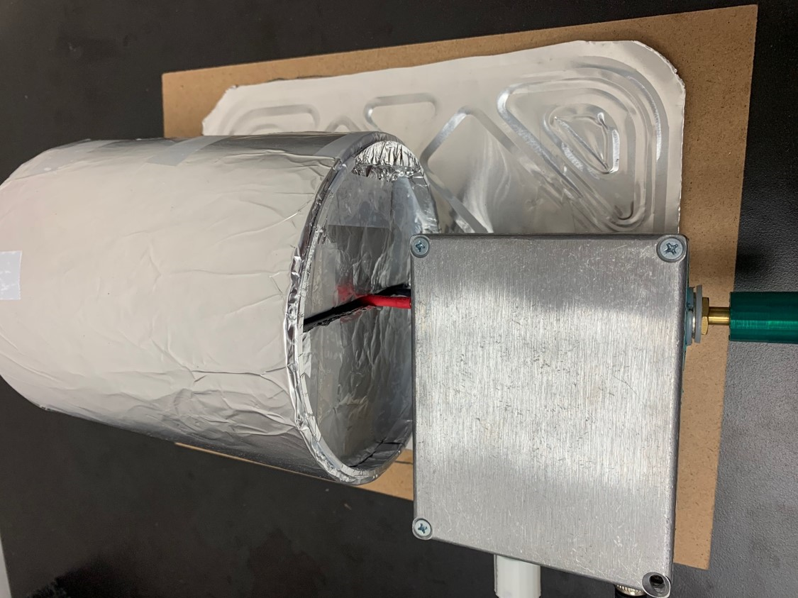
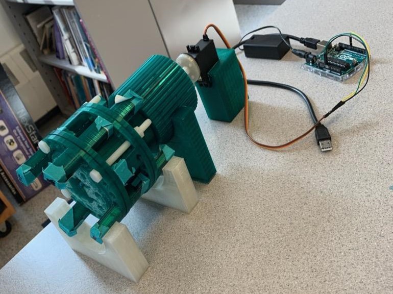
An image of the full gradient setup, as well as the sample rotator.
To further our Mandhala array optimization, we again used the gaussmeter to take swathes of measurement pertaining to the strength of the several magnetic arrays our setup uses. We discovered where, in the bore of our array, the magnetic field most closely matched the frequency our transceiver was tuned to. We did this in order to find the best place to place a sample to get a signal, and more importantly, how to do this consistently. We also measured the strengths of our inner array at two temperatures to try and understand if and how temperature was affecting our system. There were some temperature differences, but they changed in a fairly consistent way so our optimization protocol for arranging the magnets in the Mandhala would still be helpful. (See the blog post on optimizing the NMR Mandhala from 2019 for more information.)
Conclusion
This summer was a huge leap forward. The team managed to detect some (fake) signal from our system, which was one of the main goals. However, there is still plenty of work to be done, and next summer other students will pick up where Jon and Aaron left off, excited to fulfill Merideth’s goal of making MRI technology more accessible and affordable.