(Written by Jonathan Sheppard)
Intro
This summer the team took the previous year team’s RF probe design and both updated and upgraded it, in an attempt to optimize its functions. As with last year’s design, we used the text Experimental Pulse NMR: A Nuts and Bolts Approach by Eiichi Fukushima and Stephen B. W. Roeder as a guide. The main sections used will be noted throughout this post.
As noted in the previous post, below are some general guidelines on the inductor coil specifications (from the section “V.C.4. Probes” (p. 373-385)): * A good coil for RF probe has a large inductance, which is given by the equation: $$L=\frac{n^2a^2}{23a\ +\ 25b},$$ where $n$ is the number of loops, and $a$ and $b$ are the radius of the loop and the length of the coil measured in centimeters. * The spacing between the turns of the coil should approximately equal to the diameter of the wire. * AWG14 wire is about the smallest that can be recommended for a free-standing coil.
To begin the process, we had to choose a desired resonance frequency for our coil. We brought it down from last summer’s 21 MHz to 18.75 MHz. Then, we had to note the range of capacitances the capacitors in our lab have: 10-1000 pF. Using these values, we used the formula for angular resonance: $$\omega_0=\frac{1}{\sqrt{LC}},$$ solving for $L$, to find the theoretical maximum inductance our could have: 7.2 µH.
We wanted to fit the coil inside the bore of our magnet, which has an inner radius of 1.7 cm, and also we wanted the length of the coil, $b$, to be at least 2.5 cm. Variable $a$ is the inner radius, so we subtracted the wire width (thickness) from our total 1.7 cm diameter. In theory, this would have been 1.37 cm. In practice, this became 1.1 cm. Thus, 1.1 is also the diameter of the tube we will be using to wrap our wire around. So, our $a$, which is the inner radius, is 1.1 / 2, giving $a$ = 0.55 cm.
We then chose our $b$ to simply be the length of our bore, 5 cm. Following the advice of A Nuts and Bolts Approach, we experimented with using both AWG14 and AWG12 copper wire, as our inductor coil would be free-standing. We settled on AWG14 (with nominal wire diameter 1.628 mm) due to the lowered requirements of our $b$ to achieve the highest possible inductance, $L$.
Using a python script, we created, we discovered the rest of our values needed to create an inductor coil. These values included $L$ (estimated inductance), $n$ (number of turns), $l$ (length of copper wire needed), $R$ (resistance of our length of copper wire), $Q$ (quality factor of our inductor coil), $C_t$ (tuning capacitance), and $C_m$ (matching capacitance). We’ll continue this post by walking through the equations used to get these values.
To begin, we used the following function: $$n=\frac{\sqrt{(23a\ +\ 25b)\ \ast\ L}}{a},$$ which you’ll notices is the equation we used to calculate the maximum inductance, solved for number of turns, $n$.
   1. def findL_n(a, b, d):
   2.     wireWidth = 1000
   3.     L = 0
   4.     while wireWidth > d:                  #width in cm
   5.         L += .01
   6.         n = sqrt(((23 * a + 25 * b) * L)) / a
   7.         wireWidth = b / (2 * n)
   8.     return L, n                             #L in μH
We started with a ridiculously high $wireWidth$ and an inductance, $L$, of zero. Then, we increment $L$ up in each loop, updating the $wireWidth$ each time, until our wireWidth is equal to $d$ (1.628 mm, for our AWG14 copper wire). When the wireWidth is equal (or greater than) our actual wire width, the loop breaks, returning the $L$ given by the parameters we’ve chosen. In this case, we are given our number of turns as well. Using this function, we got back $L$ = 0.52 µH and n = 15.5.
The next step was to find out how much copper wire we’d need to create the inductor coil. To do that, we needed to use our inner radius $a$ and the number of turns $n$.
   1. def findCoilLength(a, n):
   2.     return 2 * pi * (a / 100) * n
This function makes use of multiply the circumference of each loop (converting a to meters so that our output will be given in meters), by the number of loops. The output here was $l$ = 0.53 m.
Here we needed to make a quick check on our calculation. The length of copper wire used must be lower than an eighth of a wavelength at resonance.
   1. def isCoilLengthOkay(a, f_0, n):
   2.     eighthWavelength = c / (8 * f_0)
   3.     l = findCoilLength(a, n)
   4.     return l < eighthWavelength
To do this, we used the formula for wavelength, multiplied by 1⁄8 to get, you guessed it, an eighth of a wavelength. Then we simply called the function we defined before, and compared the two, and out l passed the check.
Next, we needed to find the resistance of our length of wire in order to calculate a quality factor, $Q$.
   1. def findCopperResistance(l, d):
   2.     return 4 * l * 0.0171 / (pi * d**2)   #d in mm
   3.
   4. def findQualityFactor(f_0, L, R):       #L input μH, converted to H
   5.     w_0 = 2 * pi * f_0
   6.     return w_0 * L * 10**(-6) / R
Using the formula for copper resistance: $$R=\frac{4l\rho}{\pi d^2},$$ where $l$ is the length of wire used in meters (0.53 m in our case), $d$ is the nominal diameter of wire in millimeters (1.628 mm in our case), and $ρ$ is the resistivity (0.0171 Ω*mm2/m for copper). The function estimated our coil to have an $R$ = 0.0044 Ω. Then, plugging our $R$ into the second function alongside our angular resonance frequency, ω0, and inductance, $L$, using the equation $$Q=\frac{\omega_0L}{R},$$ we get a $Q$ = 14,028. In practice, this is much lower, as will be shown later.
Finally, we use all the information collected so far to calculate how much capacitance our tuning and matching capacitors ($C_t$ and $C_m$ respectively) should have.
   1. def findC_t(f_0, L):                    #L input μH, but converted to H
   2.             w_0 = 2 * pi * f_0
   3.             return 1 / (L * 10**(-6) * w_0**2)
   4.
   5. def findC_m(f_0, L, R):                 #L input μH, but converted to H
   6.             Q = findQualityFactor(f_0, L, R)
   7.             C_t = findC_t(f_0, L)
   8.             w_0 = 2 * pi * f_0
   9.             return sqrt((Q * w_0 * L * 10**(-6) * C_t**2) / 50) - C_t
Our tuning capacitor simply required us to solve our angular resonance equation for $C$, this time, instead of $L$. Our matching capacitor required a bit more work, but it was simple enough. We used an equation given by A Nuts and Bolts Approach, solved for $C_m$: $$R\ =\ \frac{Q\omega_0L{C_t}^2}{{(C_m\ +\ C_t)}^2}.$$ This function gave us a $C_t$ of 138 pF and a $C_m$ of 180 nF.
Summary of Coil Design Process
Thus, we had all the specifications we needed to create an inductor coil to suit our needs. Below is a quick summary of all of the values above, so they’re all in one place and also to refresh your mind of them. Keep in mind these are theoretical values received from our python script. Not all of them stayed the same, as theory and practice are separate beasts.
| $f_0$ = 18.75 MHz | $L$ = 0.52 μH | $Q$ = 14,028 |
| $\textrm{Max }L$ = 7.2 μH | $b$ = 5 cm | $n$ = 15.5 |
| $R$ = 0.0044 Ω | $C_t$ = 138 pF | $d$ = 1.628 mm |
| $a$ = 0.55 cm | $l$ = .53 m | $C_m$ = 180 nF |
RF Probe Circuit Design, Building, & Testing
In accordance with A Nuts and Bolts Approach, we used the parallel tank circuit suggested on page 381.
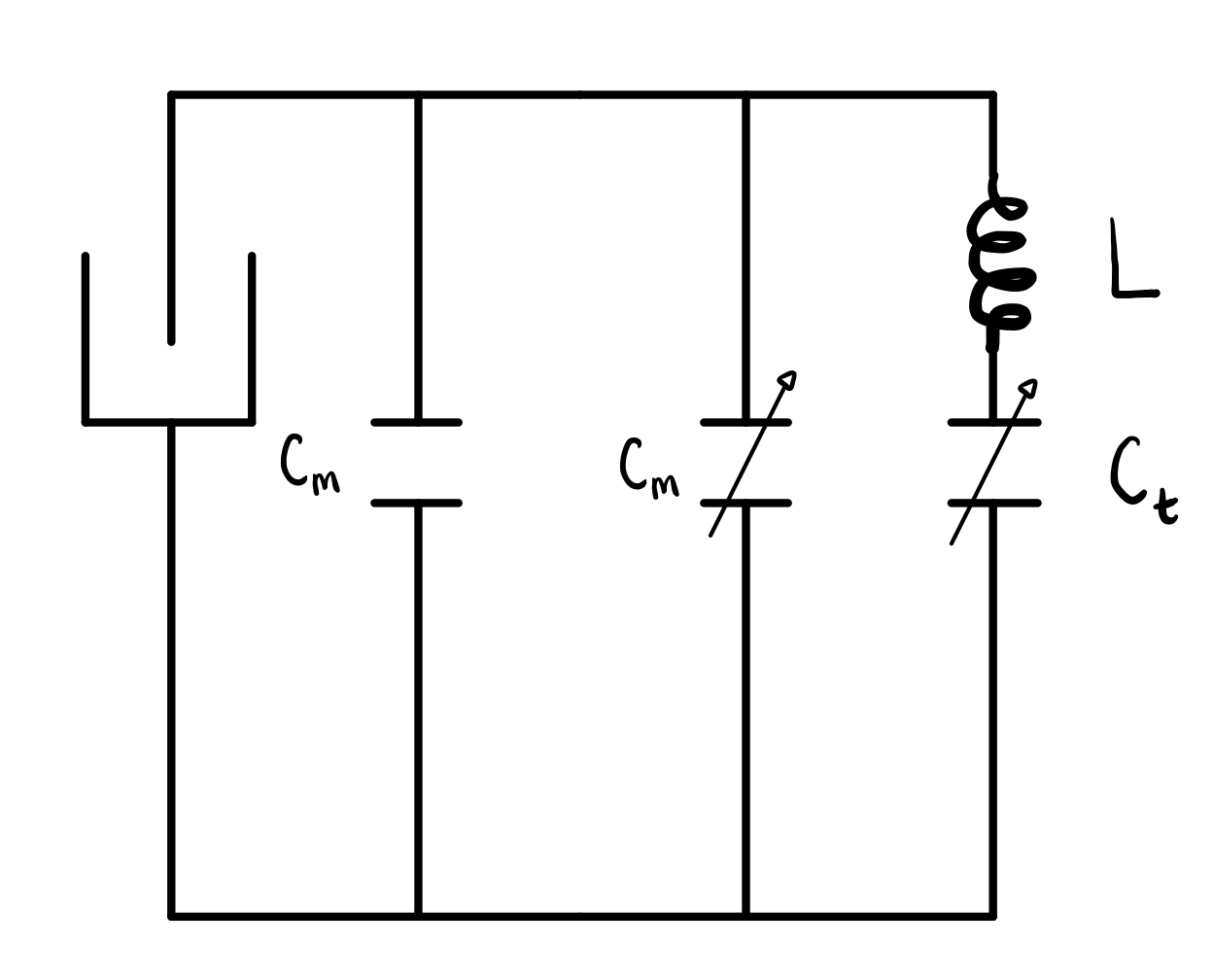
This design is a bit different than last summer’s, due to the fact that we more closely followed the route suggested in A Nuts and Bolts Approach. Another difference, and one that is a bit more fundamental to the design, was to future-proof it. This came in the form of making the circuit Plug-and-Play. Before, everything, including the inductor coil and BNC cable, were hardwired into the circuit. This required the BNC cable to be spliced and soldered into the circuit. The new design made use of a BNC connector (no more destroying BNC cables) and banana clips for the inductor coil. This meant we could use varying lengths of BNC cable, depending on the situation, and that we could also try out different coils if necessary. In the second version of the design, we even added a clip for the static matching capacitors, so those could be clipped in and out at will with ease.
Another design change came in the form of the coil design. The previous year’s design created an inductor coil inside of a test tube, which in turn would fit into the bore of the magnetic field. This updated design puts the inductor coil on the outside, with no tube to fit in other than the bore itself. This would have increased the room we had for samples, if not for the fact that we upgraded to AWG14 wire from AWG18; hence, any gains were offset with the thicker wire.
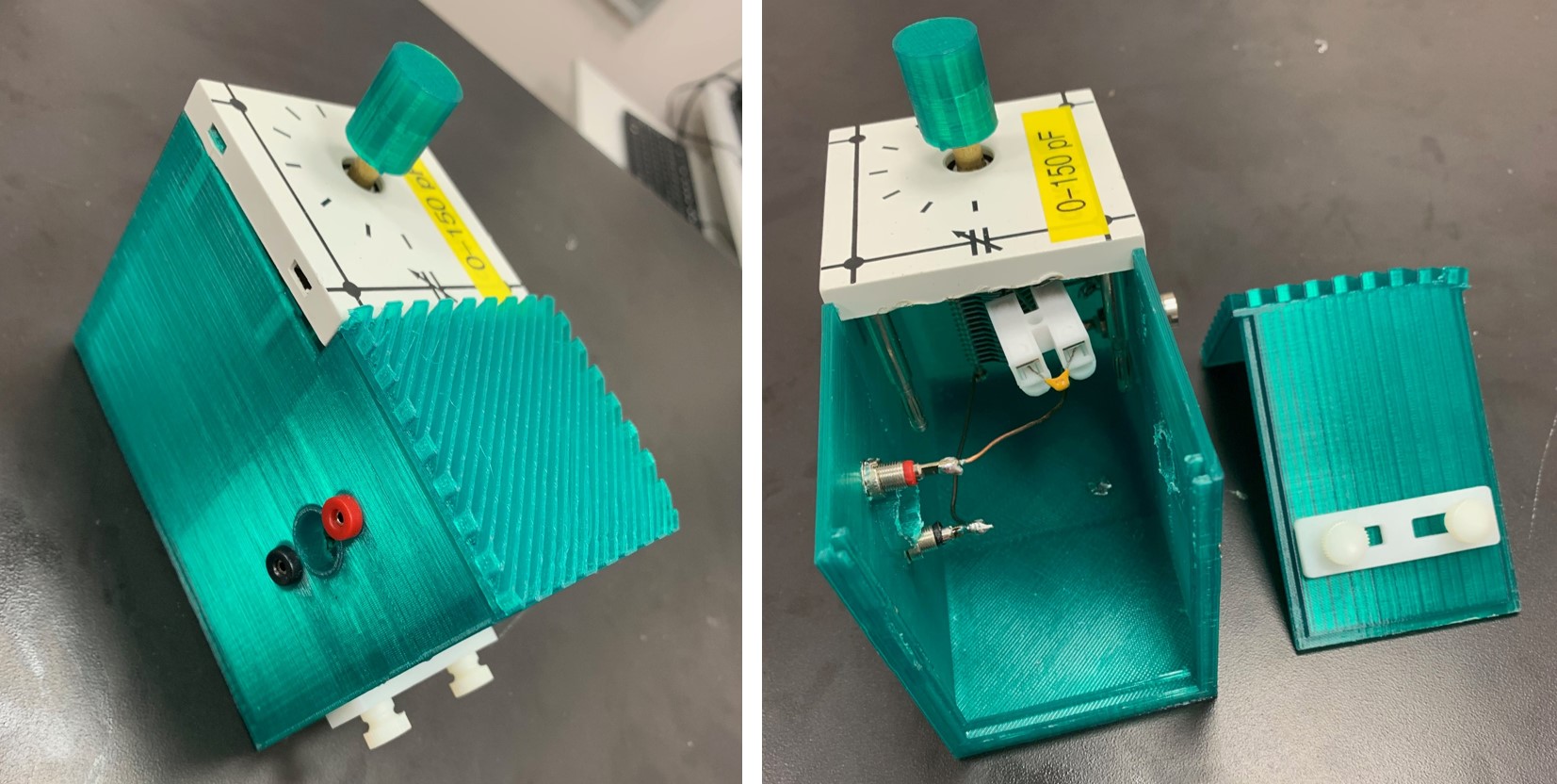
And finally, the last design change came by turn the coil perpendicular to the rest of the circuit. This was due to the fact that a final form of our machine would ideally have a flow system in place to let a live Zebrafish be imaged. To do this, the flow system would have to run through the bore (and hence through our inductor coil) on both sides. So, twisting the inductor coil perpendicular allowed us to craft a tube (or simply two holes in the second design variation) through which the flow system would snake through, without hitting any circuitry and impeding our RF Probe.
Pictured to below is the first complete design using these new thoughts. It was completely 3D-printed with the exception of the white cap we salvaged and bolted our own variable capacitor to. We found a good tuning capacitance at 72 pF, and continued to test different matching capacitances.
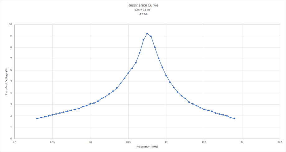
The graph below is one of the resonance curves for matching capacitance of 100 nF, with the accompanying quality factor.
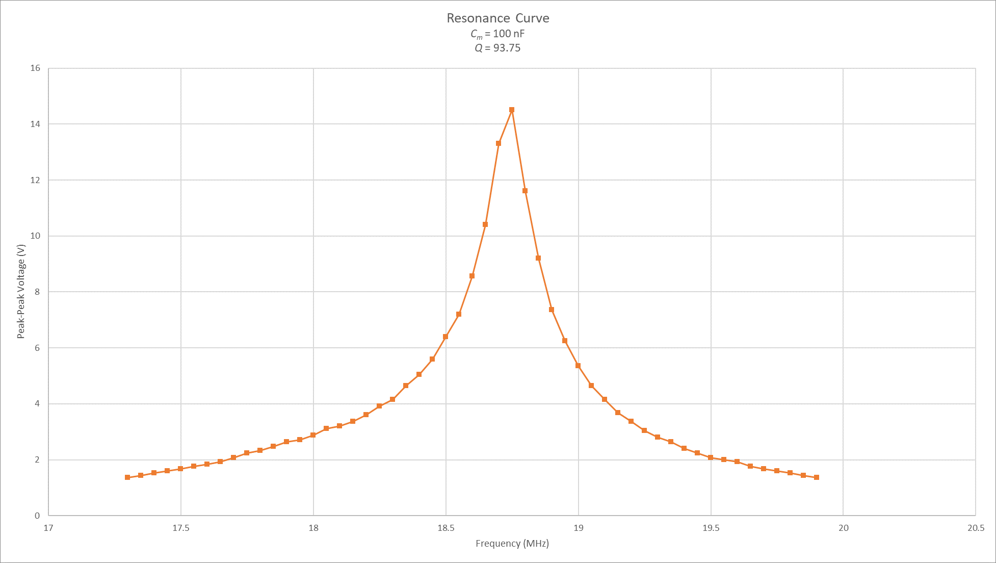
When the testing began, the resonance frequency was quite a bit lower than we wanted. By changing the matching capacitance, we managed to get it around 18.75 MHz, which was our desired resonance frequency. In this design, the matching capacitors were hard-wired into the circuit, so each test required soldering to modify the capacitors. In the picture above, you’ll notice the snap connector. After building an aluminum version (more on this in the next), we learned that this was a much simpler method of changing our static matching capacitors.
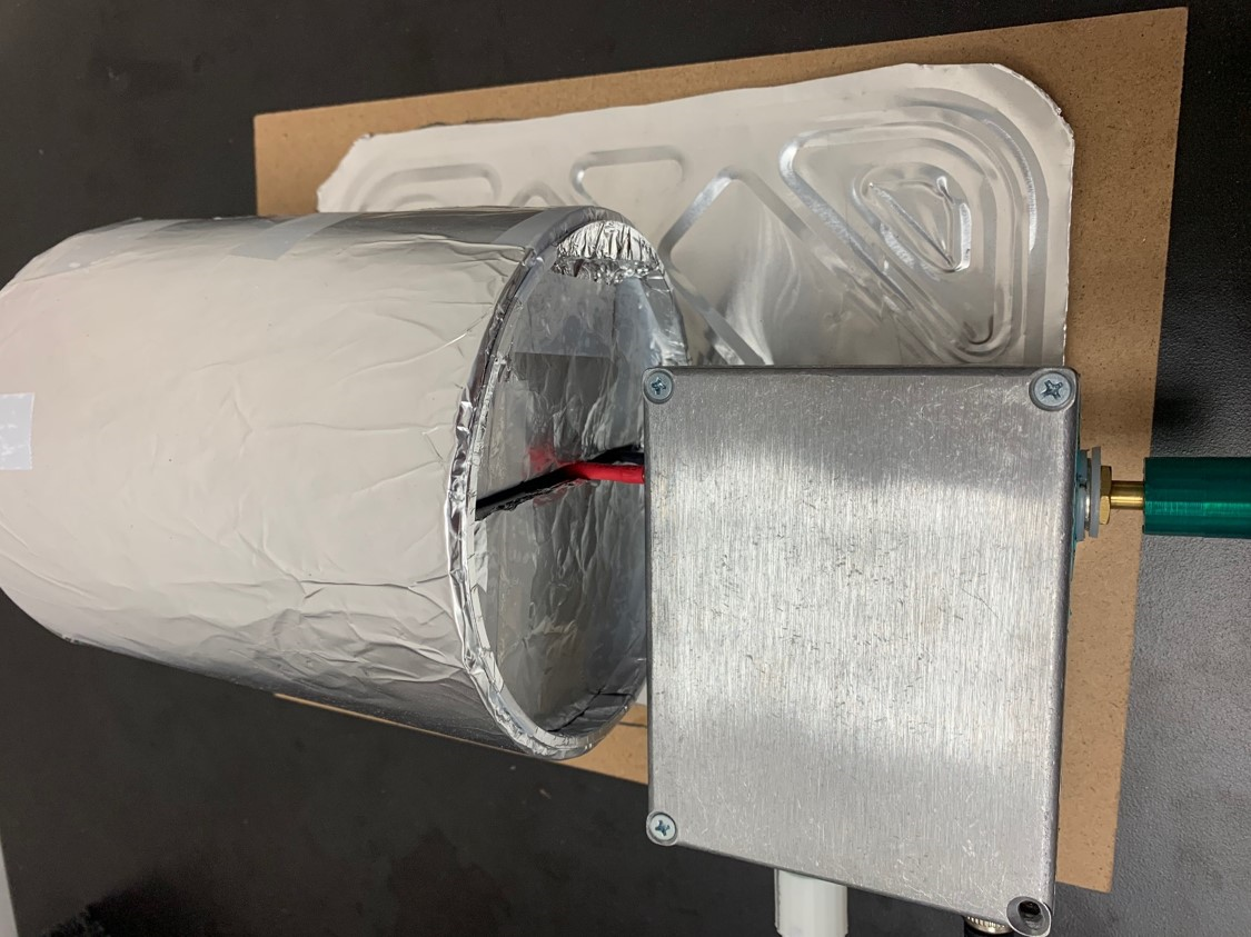
As a first design test, things went surprisingly well. However, we were seeing some odd background noise. To combat this, we decided to try again, replacing our plastic, 3D-printed enclosure for a shielding aluminum one, pictured below. The circuit was essentially the same, and we used more variable capacitors for both the tuning and matching, in addition to the static capacitors in parallel with the matching. The only change came in the form of the matching capacitor. We added a small spring connector (in keeping with our Plug-and-Play mentality), so that if we wanted to further experiment with the matching capacitance, we wouldn’t have to solder over and over again, improving the quality control of subsequent tests. An important thing to note is that, due to the banana clips, we were able to use the exact same inductor coil as our last model was tested with.
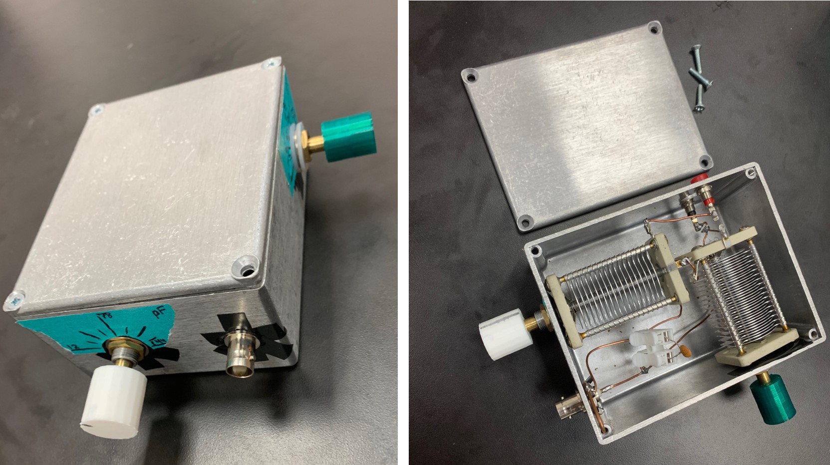
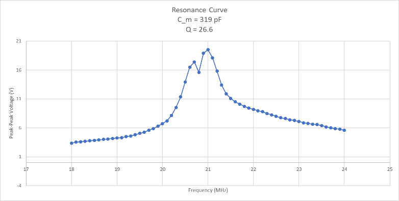
We also noticed that our matching capacitance was much too high. The TeachSpin system had a static matching capacitor of approximately 900 pF, with variable capacitors equaling 330 pF. Knowing that our system was similar to the TeachSpin (and that it was the TeachSpin we were trying to emulate) we lowered our static matching capacitor from nanofarads to picofarads, and began to see better peak-peak voltages. This went against our python program, and against our working theory. On possible explanation is that the resistance in reality is larger than the calculated resistance of the copper wire. This is exemplified below in the resonance curves, the first has a large matching capacitance and the second has a lower one. The third curve was taken with an Analog Discovery 2 System Analyzer using the SpinCore RF processor to generate a fake signal (rather than the TeachSpin synthesizer and an oscilloscope). This fake signal consisted of a 5 Vpp pulse that was 25 μs long and repeated every 50 μs. The last curve was generated using the same setup, except we used the TeachSpin magnet and RF tank circuit instead of our own.
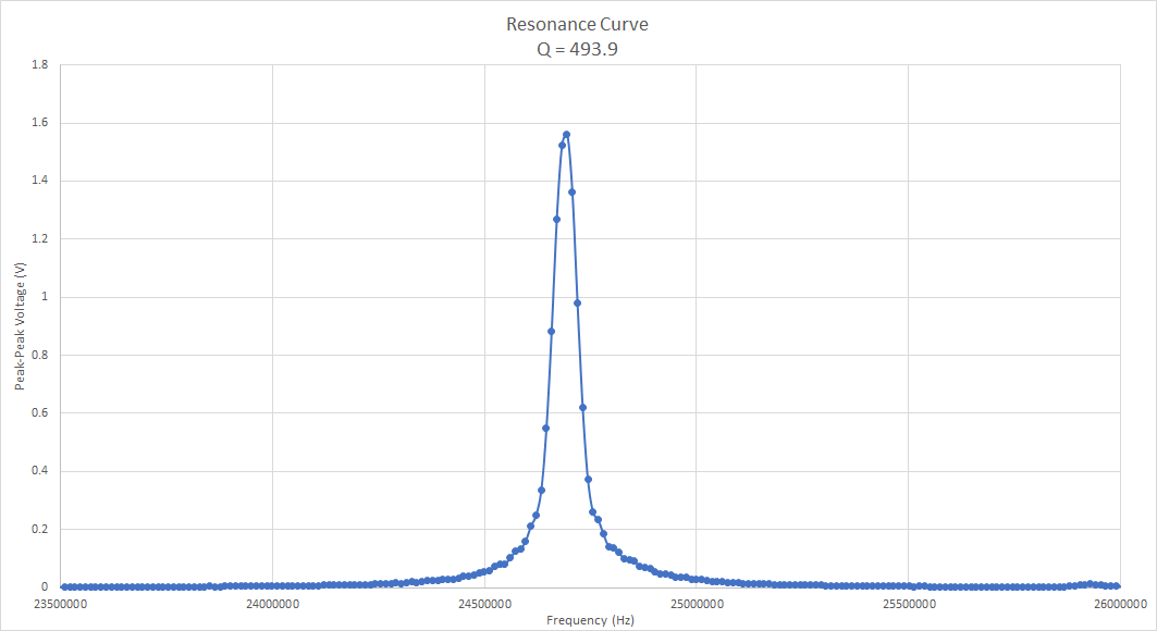
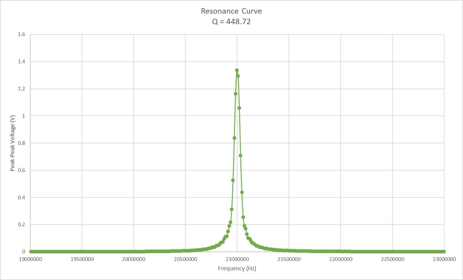
NOTE: The final two curves are not resonance curves, they are the amplitude of the fake signal at the tuned frequency is being detected. (To get a resonance curve, one would need to change the frequency of the fake signal and plot the amplitude of the response curve relative to the change in frequency.)
We tried using the TeachSpin receiver to measure the response to a fake signal generated by the SpinCore RF processor, but kept on getting very noisy signal with a large baseline and barely visible pulse. We hypothesize that this bad data was due to the receiver on the TeachSpin `subtracting out’ the RF frequency before output. The SpinCore RF processor is not synced with the TeachSpin so this subtraction process would not be very successful. However, the fact that our tank circuit’s sensitivity is comparable to the TeachSpin’s is notable.
Before we began to use the Analog Discovery system, we were still seeing the same noise that we noticed with our 3D-printed version. In another attempt to lessen this noise, we crafted some rudimentary shielding to encompass our system. Importantly, we also had to ground the actually body of our enclosure, and, when connected to the shielding system, this allowed our shield to become grounded as well. Without grounding, our shield wouldn’t give us much noise reduction. As in all things with this project, our goal was to match or surpass the TeachSpin system. Surprisingly, our shielding (shown below surpasses the TeachSpin system ever so slightly in its ability to reduce noise.
The big, end goal of this summer was to get some sort of signal from our system. Unfortunately, we were unable to achieve this goal. However, the sheer amount of progress we were able to make in other areas more than makes up for this. We have several designs for new circuit enclosures. Said designs are consistent and reproducible, with implementations for ease of access, such as adding banana clips to the inductor coil and using a snap connector for the static matching capacitors. We made real progress with figuring out how to use both the RF Processor and Analog Discovery System Analyzer. Used in conjunction with each other, we are well on our way to acquiring signal not dissimilar from the TeachSpin System.
One of the things we’re looking forward to working on next summer is obtaining a directional coupler to further our utilization of our RF Processor and Analog Discovery Analyzer. We will also be building a transmit/receive circuit so that we can use our magnet, RF probe, and the RF processor to be completely independent of the TeachSpin system.