This work was a follow-up to the work discussed in the previous post from 2018 on optimizing positions of magnets in the NMR MANDHALA based on a close reading of of Soltner and Blumler’s 2010 article “Dipolar Halbach Magnet Stacks Made from Identically Shaped Permanent Magnets for Magnetic Resonance”. There the dipole approximation is used for each cubic magnet in order to optimize magnet position to take into account inhomogeneities in the magnetic moments of the magnets used in the Mandhala (see ‘Variation of Magnet Properties’ section of article).
The article creates a ‘cost function’ that measured the deviation of the magnetic field at the center of the Mandhala from what one would get if all the magnets were exactly identical with magnetic moments equal to the mean of the magnets being used. This ‘cost function’ approximates that all the magnets contribute to the field as ideal magnetic dipoles, which works well in the far-field case. One then tries all possible permutation of magnets in each of the available spots, and saves the configuration with the minimal cost function.
We noted that our previous implementation of this method is good at finding a configuration where the magnetic field at the center is close to the average magnetic field one would expect from the given magnets, but that this condition can be met by having a symmetric gradient of the magnetic field in the 2D plane (e.g. higher fields on one side, lower fields on the other, the center field being exactly average).
In our updated optimization procedure:
we adjust the cost function to sum the field deviation over the center and a circle of points around the center in the central 2D plane in the imaging volume of interest.
we give an estimate for the magnetic moments of the bar magnets and use constants to calculate an estimate for the magnetic field strength we should get from our Mandhala setup
We did this optimization separately for the tall Mandhala (using 2” tall magnets) and the center Mandhala (using 1” tall magnets). Below is a figure comparing the magnetic field mappings for the taller Mandhala with center Mandhala using 2018 optimization method (left) and the opimization method described above (right):
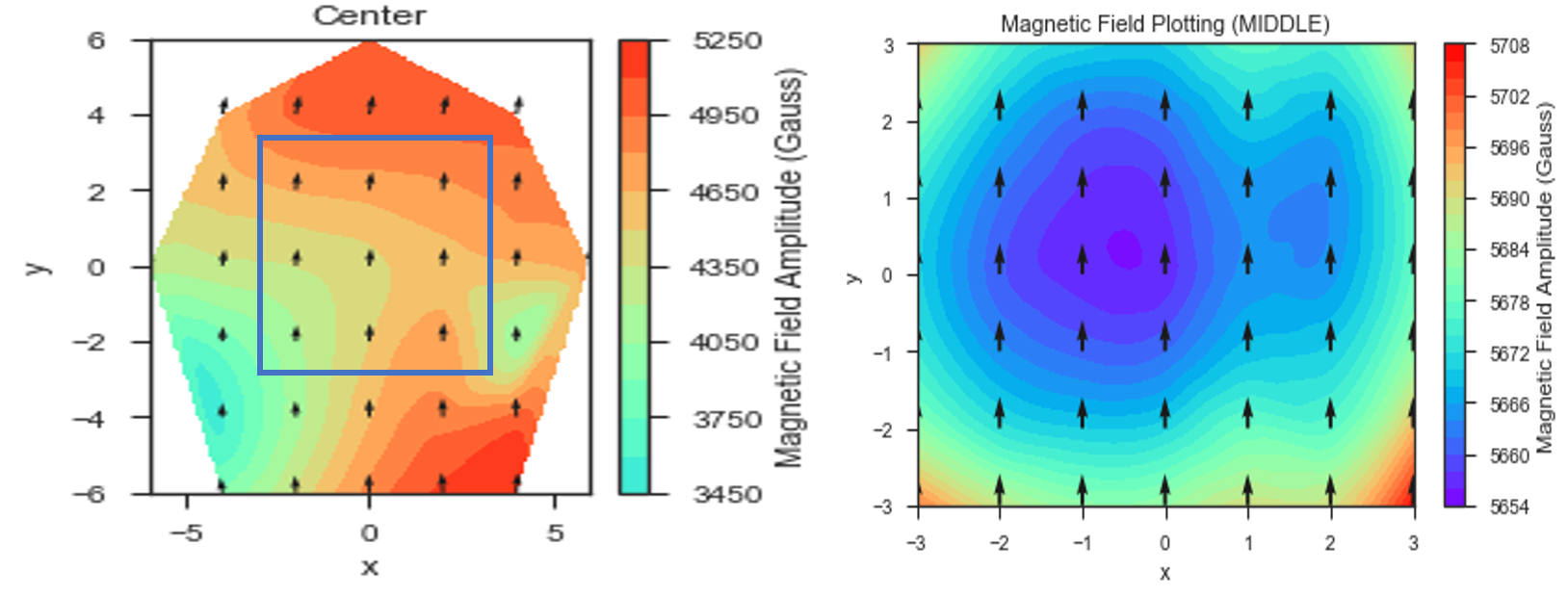
As can be seen the homogeneity is much better (a range of 54 Gauss over the 3 x 3 mm region measured instead of 1050 Gauss). The magnetic field also has more of the radial symmetry we would expect from the Mandhala. The overall magnetic field strength is also increasing as we learn how to better optimize our field with our given permanent magnets.
For a nice annotated Jupyter notebook providing the code we used for optimizing our Mandhalas, see the EvenMoreOptimizedMandhala_2019.ipynb in the `SLC Research’ GitHub repository.
Possible future steps:
This calculation over-estimates the magnetic field (e.g. it estimated 0.74 +/- 0.01 Teslas for inner and outer Mandhalas combined), because we are assuming the magnetic field contributed by each bar magnet is equal to a magnetic dipole with the same magnetic moment as the bar magnet centered at the center of each magnet.
It would be more accurate to break the bar magnet into cubic pieces of the same magnetization and treat each cube as a magnetic dipole. Since the magnetic moment of the bar magnet scales with the volume, breaking the 1-inch longer magnet into 3 1⁄3”-cubes would reduce each cubes magnetic dipole moment by 3 and each cube’s contribution to the field would be smaller than assumed here due to slightly increased distance from the center plane.
Could see if making such an adjustment to our model would more accurately predict the magnetic field we measure with the actual magnets (and allow us to more accurately optimize our magnet design).
Similar theory can then be applied to our permanent magnet gradient designs.